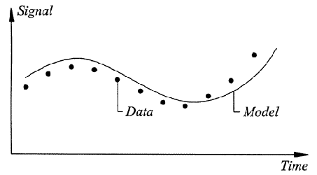
In the Stochastic Subspace Identification (SSI) techniques a parametric model is fitted directly to the raw times series data. A parametric model is a mathematical model with some parameters that can be adjusted to change the way the model fits to the data. In general, we are looking for a set of parameters that will minimize the deviation between the predicted system response of the model and measured system response (measurements). This process is often called model calibration. See the following picture

All known linear and time-invariant time domain modal identification techniques can be formulated in a generalized form as an innovation state space formulation

where the A-matrix contains the physical information, the C-matrix extracts the information that can be observed in the system response and the K-matrix contains the statistical information. The statistical information allows for a covariance equivalent modeling, so that the model can have the correct correlation function and thus also the correct spectral density function.
The number of parameters in the model is essential. If this number is to small, then the dynamical- and statistical behavior cannot be modeled correctly. On the other hand, if the number is too high, then the model becomes over-specified resulting in unnecessary high statistical uncertainties of the model parameters.
So the art of parametric model estimation is to determine a model with a reasonable number of parameters. This means that what you must do when you are estimating state space models is to choose the model order also known as the state space dimension, which is the dimension of the A-matrix.
ARTeMIS Modal has five different implementations of the Stochastic Subspace Identification technique. These are:
Unweighted Principal Component (SSI-UPC)
Extended Unweighted Principal Component (SSI-UPCX)
Principal Component (SSI-PC)
Canonical Variate Analysis (SSI-CVA)
Unweighted Principal Component Merged Test Setups (SSI-UPC Merged)
The four first are all working per Test Setup. This means that you extract the modes for each Test Setup and then use a tool called Select & Link to merge the results to form a global set of modal parameters. The fifth technique do the merging as a part of the signal processing done in the Prepare Data Task, and the result is that you work with this tool as if there was only a single Test Setups even though there are multiple Test Setups. This technique is dedicated to multiple Test Setups.
See the Technical Paper on the Stochastic Subspace Identification Techniques for a more comprehensive description about how the Stochastic Subspace Identification techniques work and what the mathematical difference between the implementations are.
When the stochastic state space system is being estimated using e.g. the Stochastic Subspace Identification techniques we obtain what is called a realization of the true but unknown system. So the parameters of the state space system

is only estimates of the true system. You will never be able to estimate the 100% correct parameters but you can indeed estimate very accurate parameters by not using a too large state space dimension.
The above system is shown in time domain but can of course also be represented in frequency domain by its transfer function H(z) as below

where z is a frequency dependent complex number. By a complex transformation of this transfer function using the eigenvectors of A the modal decomposed transfer function appear as

This representation of the transfer function expose all the modal parameters. From the eigenvalues µjdefined as the diagonal elements of the matrix


In this equation T is the sampling interval.


For this reason this vector is called the initial modal amplitude. Since this vector describes how the white noise is distributes in modal domain, this vector describes the statistical part of the modal decomposition. All the other modal parameters relates to the dynamic system and are therefore deterministic parameters that should not change if the excitation changes.