Each Stochastic Subspace Identification (SSI) method in ARTeMIS share the same properties and the estimation window.
Modal Estimation window
Below the editor window is shown after loading a project called Plate with Harmonics.
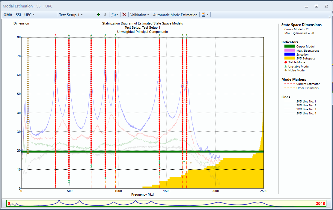
The window is divided vertically in two. On the left a stabilization diagram is shown and on the right a legend with information about the stabilization diagram is presented.
The stabilization diagram is an engineering tool used to handle bias errors in the estimates of modal parameters, considering the order of the system is unknown. The system order determines the size of the eigenstructure of the system. In the context of subspace-based system identification methods, it relates the number of poles in the state matrix to the number of identified modal parameters. Different system orders result in different estimates of the modal parameters that may vary depending on the selected order. Among those parameters there exist some that correspond to non-physical, noise and mathematical poles. Conversely to the physical poles, which are stable in the stabilization diagram, the spurious estimates have high dispersion, based on which they can be discarded from a further analysis, this will be elaborated later.
The horizontal axis is a frequency axis ranging from zero to the Nyquist frequency. The vertical axis lists the dimensions of the available state space models. This range goes from 1 to the maximum state space dimension specified in the Signal Processing configuration.
Stabilization diagram and modal alignments
The problem of parametric model estimation is that the true system order is unknown. The way to overcome this is to estimate a range of candidate state space models, that result in groups of modal parameter estimates that can be clustered into so-called modal alignments and later on to stabilization diagrams by some practical criteria, like the relative difference between the consecutive parameters and the modal indicators. Thus one modal alignment is a group of modal parameters that correspond to one mode and are estimated for a range of system orders. They are aligning themselves (hence the name) with respect to a mode according to some criteria. A group of modal alignments of some selected parameters, like natural frequencies, forms the stabilization diagrams,
Hereafter the properties used to create stabilization diagrams are outlined.
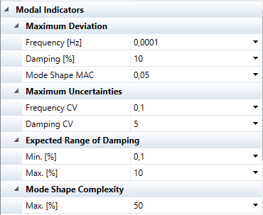
- Maximum Deviation:
This property sets a limit for a maximum deviation for modal parameters in one modal alignment.
- Maximum Uncertainties (SSI-UPCX only):
This property sets a limit for a maximum uncertainty, that is the Coefficient of Variation (CV), for modal parameters in one modal alignment.
- Expected Range of Damping:
This property sets a limit for a maximum range of damping ratio estimated with the chosen system identification technique.
- Mode Shape Complexity:
This property sets a limit for a maximum mode shape complexity factor (MCF) estimated with the chosen system identification technique.
Thus a stable mode of a model is one that compared with one of the estimated modes of the previous model fulfill the union of the following requirements:
- maximum allowed deviation of the natural frequency of the mode when compared with one of the modes of the successive model
- maximum allowed deviation of the damping ratio of the mode when compared with one of the modes of the successive model
- maximum allowed deviation of the Modal Assurance Criterion (MAC) of the mode shape vector of the mode when compared with one of the modes of the successive model
- maximum Coefficient of Variation (CV) of natural frequency and damping ratio. CV is defined as the standard deviation of the estimate divided by its value (SSI_UPCX only)
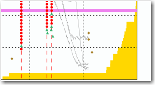
If the deviations of all the above requirements of a mode is less than the specified maximum allowed deviations then a mode is characterized as stable and will be marked with a red cross.
If one or more of the above requirements are not fulfilled then the mode is characterized as unstable and will be marked with a green diagonal cross. So by decreasing the maximum allowed deviation the number of candidate models will also decrease. The setting of the requirements are performed in the Modal Indicator section of the Properties window.
Eliminating Harmonics and Noise Modes
When a state space model is estimated from measured data not only structural modes will be estimated but also so-called noise (computational) modes. These noise modes are used by the algorithms to account for non-fulfilled assumptions. Noise modes appear e.g. in the following situations:
- Limited data records (Accounts for the violation of the infinite amount of data assumption).
- Colored noise caused e.g. by non-white excitation and / or filtering (Accounts for the violation of the assumption of having white noise disturbance only).
Typically, noise modes are spread in a non-systematic and non-repeated way. Because they usually are very heavily damped and because structural modes usually are lightly
damped we can exclude large parts of the noise modes from the analysis by looking at the damping of a mode. If the damping ratio is larger than some predefined value, say e.g. 5%, then the mode is probably a noise mode. The setting of the range of the damping ratio of a structural mode is done in the Modal Indicator section of the Properties window. Modes having damping ratios outside this range are characterized as noise modes and marked in the stabilization diagram with yellow diagonal crosses. Besides being marked they are also excluded completely from the evaluation of stable/unstable modes.
If the measurements has been acquired on a structure having rotating equipment running, then also the "modes" of this external periodic excitation will be estimated. The "modes" will contain the harmonic frequency and a damping that is extremely low. The damping is typical much lower than the one of physical modes, and can as such be used to filter the harmonics out of the analysis. This can be done by setting the lower limit for damping of physical modes to a small but non-zero value, like 0.1%. In this way the harmonics will be characterized as noise modes and left out when the global modes are estimated.
Estimating State Space Models
Before starting the estimation of state space models make sure you have enabled the estimation of the so-called Common SSI Matrix by clicking the Enable in the Stochastic Subspace Identification section:
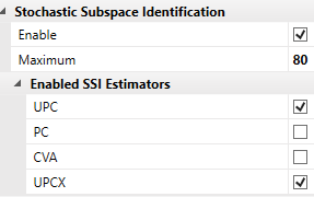
The Maximum value is actually the number of rows in the Common SSI Matrix and is equal to the maximum state space dimension that be estimated in SSI. Since this number is also equal to the maximum number of eigenvalues to estimate and since under-damped modes use two eigenvalues per mode, it means that you basically can estimate a number of modes equal to the half of this number. In the above example it means 40 modes.
Besides selecting the maximum dimension, you should also check what estimators you like to use in the analysis. By default SSI-UPC and SSI-UPCX are selected and the ones to recommend.
When you then start the Modal Estimation window for one of the SSI techniques you just need to select a Test Setup, either in the Data Organizer or in the drop down list in the toolbar of the Modal Estimation window. This will automatically trigger the estimation of all the available state space models. Once all models of the Test Setup has been estimated you will see this in the Data Organizer by a check mark next to the name of the Test Setup:
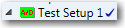
You can then repeat the selection for the other Test Setups. Once all models in all Test Setups have been estimated the software will, as a first time service, estimate the global modes and present them in the Modes list to the right.
Available Subspace of the Common SSI Matrix
The singular values (the yellow horizontal bars) indicate the rank of the weighted common SSI input matrix.
What you are doing when you estimate a state space model is to specify what subspace of singular values of this matrix to include in the estimation. This subspace should at least include all singular values significantly different from zero. This means all the ones that look yellow in the diagram.
Crystal Clear SSI
By default the estimator used to obtain the state matrix is a modified least squares solver called Crystal Clear SSI. This estimator require some extra information about the number of eigenvalues that are significantly present in the data. By default the estimator figures this out by looking at the singular values. Once a singular value is only a certain fraction of the first one the number this singular value has, counting from the first one, is normally a good approximation for the number of significant eigenvalues. You might also insert this number manually, and can then try to count the number of significant peaks in the singular values diagram behind and multiply this count by two. This is also a good approximation normally.
The Crystal Clear SSI settings are listed in the Properties window under the Modal Estimation section:
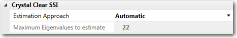
The Estimation Approach is by default set to Automatic but can be changed to Manual in which case you can specify the Maximum Eigenvalues to estimate. You can also disable Crystal Clear estimation by selecting Disable. In this case it will be the traditional least squares estimation algorithm that will be applied.
When you change these settings and hit <Return> the stabilization diagram will be update automatically.
The Maximum Eigenvalues to estimate is indicated in the stabilization diagram with a magenta colored cursor.
Cursor Model and Selection Range
There is a green horizontal cursor that you can move up and down with the arrow keys. This cursor can be used to select one model. Information from this model can then be viewed or saved.
You can view all the modal parameters of the selected model by starting the Cursor Model window from the Application Task Bar Windows drop down list.
Validation of Cursor Model
The validation of the time domain estimation of the state space models is actually performed in the frequency domain. The reason for this is that it is very easy in frequency domain to see the repeated trend of structural modes when estimating multiple state space models. But you should remember that the actual estimation behind the screen is performed on the raw time series data of the currently selected test setup in time domain.
The stabilization diagram display the frequencies of the each mode of the cursor model. This is only a fraction of information that is contained in the state space model. The Validation dropdown button in the toolbar allow you to view spectral densities of the response as well as of the prediction errors.
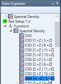
The first step is to select either a cross-spectral density (CSD) or an auto-spectral density (ASD) from the function list in the Data Organizer, see below:
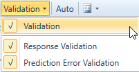
Now press the Validation dropdown button and click the Validation item to start the estimation of spectra and prediction errors.
The Estimate window will now split and the validation windows appear in the bottom:
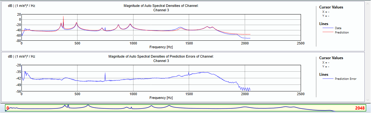
The upper diagram display the synthesized spectral densities in red as well as the spectral densities estimated from the measurements in blue. If the dynamics as well as the statistical properties are correctly estimated the synthesized spectral densities should be comparable with the spectral densities of the measurements.
The lower diagram display the magnitudes of the spectral densities of the prediction errors. The prediction errors are calculated as the difference between the measurements and the response that can be predicted by the state space model. If the model matches the measurements completely then the prediction errors forms a realization of a white noise. A white noise has a completely flat spectrum. The aim of checking the prediction errors is as such to check whether they in general are "flat" or not. In the regions where there are not flat there is a bad fit between model and data. In the above diagram especially second harmonic order around 750 Hz seems to be very poorly fitted by the model. Also the low frequency region as well as close to the Nyquist frequency the fit seems quite poor.