Compared to Frequency Domain Decomposition (FDD), the enhanced version adds a modal estimation layer. The modal estimation is now divided into two steps. The first step
is to perform the FDD Peak Picking, and the second step is to use the FDD identified mode shapes to identify the Single-Degree-Of-Freedom (SDOF) Spectral Bell functions
and from these SDOF Spectral Bells estimate both the frequency and damping ratio.

The SDOF Bell Identification

The identification of the SDOF Spectral Bell is performed using the FDD identified mode shape as reference vector in a correlation analysis based on the Modal Assurance Criterion (MAC). On both sides of the FDD picked frequency a MAC vector between the reference vector and the singular vectors corresponding to a certain frequency is calculated. If the largest MAC value of this vector is above a user-specified MAC Rejection Level the corresponding singular value is included in the description of the SDOF Spectral Bell. The search on both sides of the reference frequency is continued until no MAC values are above the rejection level. Outside the search range the values of the SDOF Spectral Bell is set to zero. This means that the lower MAC Rejection Level the more singular values are included in the SDOF Spectral Bell. However, at the same time the lower MAC Rejection Level the deviation from the reference vector is allowed. Therefore, a good compromise is to use an initial MAC Rejection Level at 0.8.

The Modal Parameter Estimation

Besides storing the singular values that describe the SDOF Spectral Bell, the corresponding singular vectors are averaged together to obtain an improved estimate of the mode shape. The average is being weighted by multiplying the singular vectors with their corresponding singular values. This means that the closer the singular vectors is to the peak of the SDOF Spectral Bell the more weight it has on the mode shape estimate.

The natural frequency and the damping ratio of the mode is estimated by transforming the SDOF Spectral Bell to time domain. What we then obtain is a SDOF Correlation Function, and by simple regression analysis we obtain the estimates of both the natural frequency as well as the damping ratio.

The estimation of the damping ratio is performed by identification of the positive and negative extremes of the correlation function. Taking the logarithm of this decaying curve will for viscous damped linear systems result in a straight line on which the damping ratio can be estimated by linear regression. However, due to broad-banded noise and / or non-linearities the beginning and end of the curve might not be straight. Such non-straight parts should not be included in the regression.

The estimation of the natural frequency is performed by a linear regression on the straight line that describes the correlation crossing times. However, again the beginning and end of the curve might not be straight and should not be included in the regression.

These modal estimates will be good if the correlation function decays to a sufficiently small level of correlation. This can be accomplished by having sufficient frequency resolution. In this case the bias of the natural frequency and the damping ratio will be small.

The EFDD Modal Parameter Estimation at a Glance

In the case of the Plate with Harmonics example the Modal Estimation window looks as below when started right after the signal processing of the data is complete:

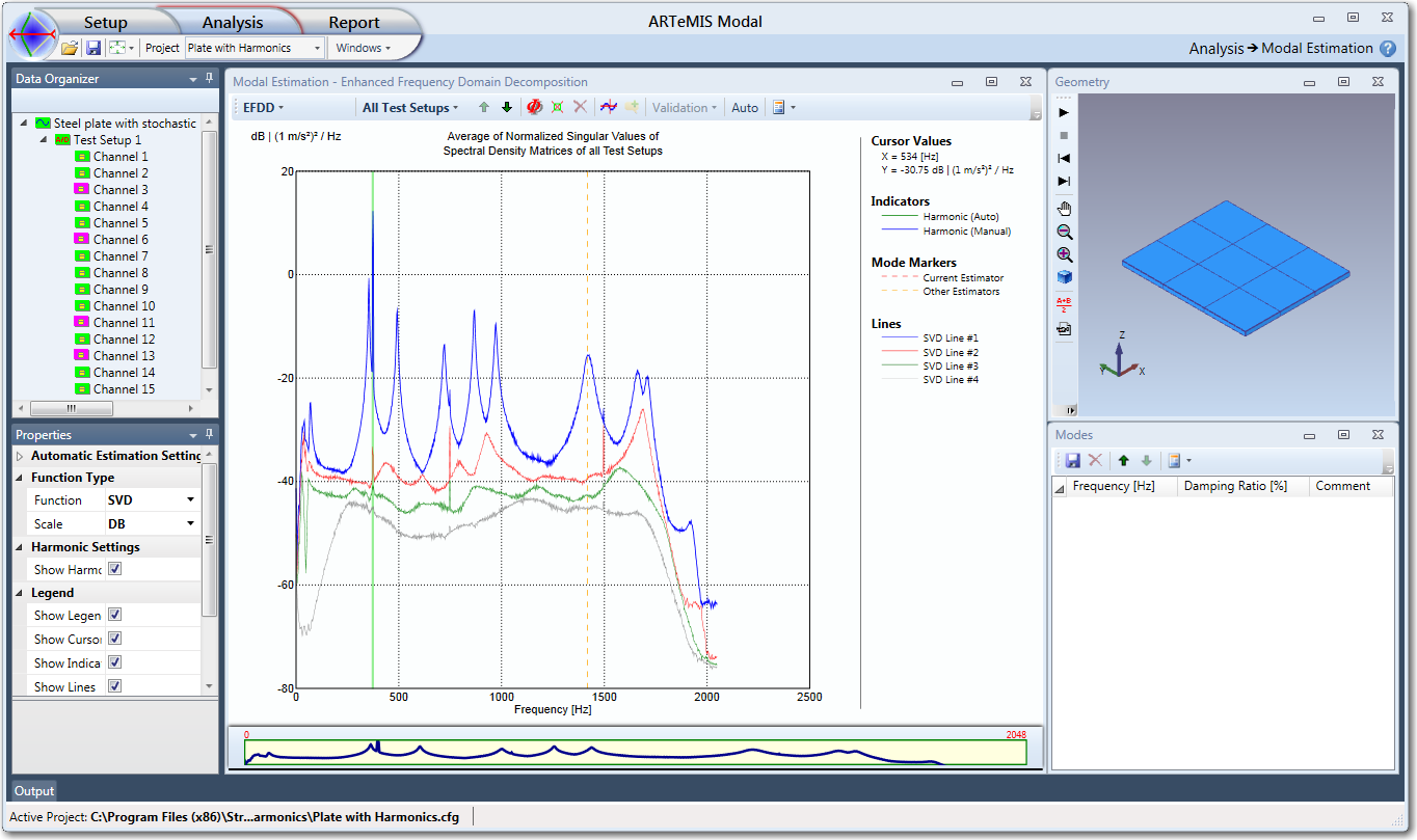
The peak picking is performed in the Modal Estimation window and the results can be verified immediately after in e.g. the Geometry window. The estimated modes can be validated and fine-tuned in the Validation window using the settings of the Properties window and they are listed in the Modes window.

As it can be seen above, the Modal Estimation Window looks exactly like the FDD Modal Estimation window and the procedure is also exactly the same. The only difference between peak picking in FDD and EFDD is that in the last technique peak picking is used not only to obtain a reference frequency but also a mode shape to be used in the EFDD Modal Estimation.

When you estimate these reference parameters you will usually get the best result by picking on top of the peaks. Here the reference mode shape estimate will most accurate in case of well-separated modes. If the modes are repeated or closely spaced you should follow the guidelines listed in the description of the FDD Modal Estimation window, for estimation of these special cases.

When you have picked a reference mode shape and frequency, as seen below, the modal parameters estimation is performed immediately with the default settings. The default modal estimation settings are edited in the Properties window in the Estimation Parameters section, that is available when a specific Test Setup is selected, see below:

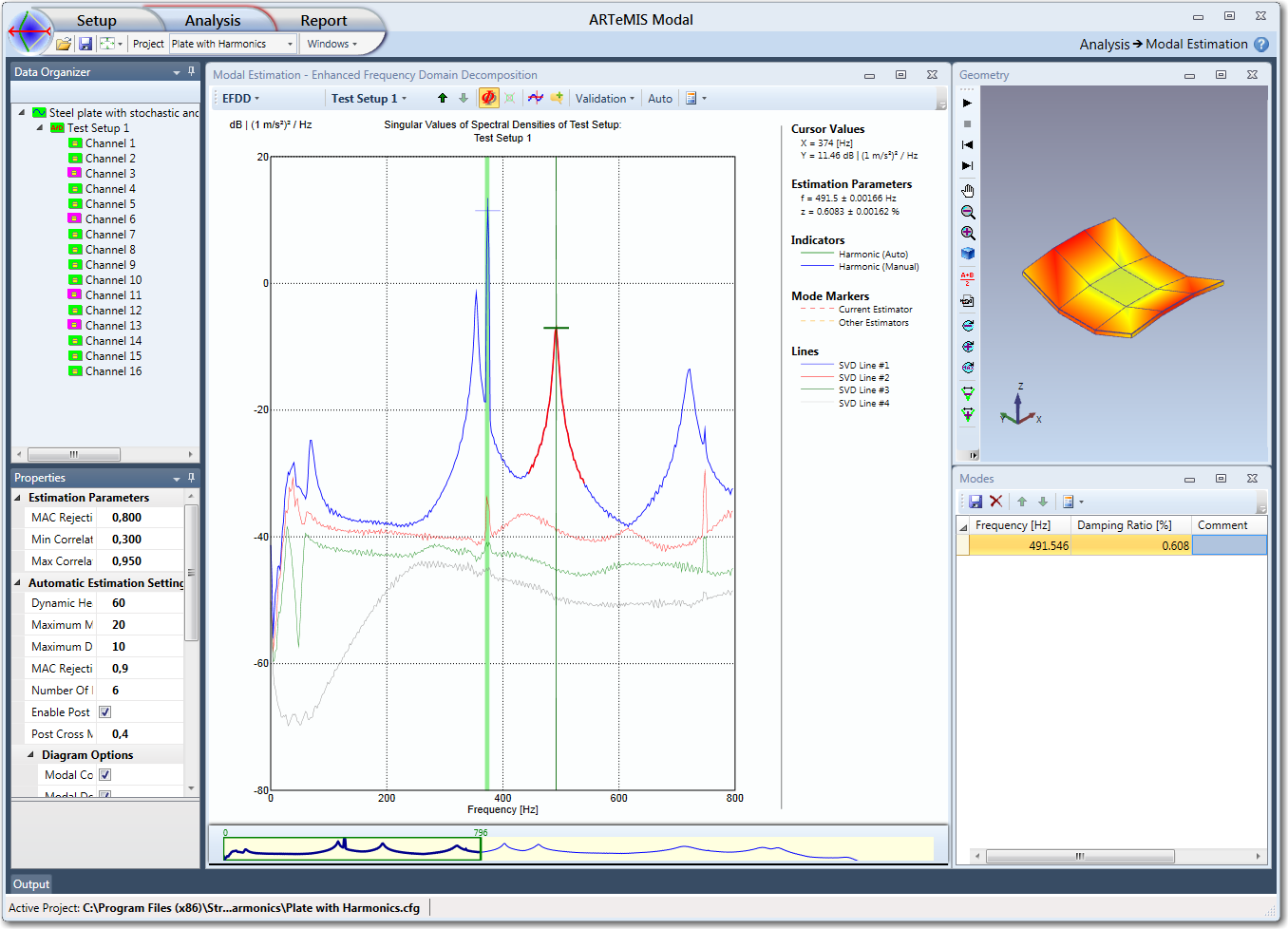
To validate the estimated mode shape by animation you click the Start Animation button  in the Geometry window. To adjust and / or validate the estimation of the natural frequency and the damping ratio, you shift from All Test Setups level to one of the Test Setups by clicking on the drop down list in the toolbar of the Modal Estimation window, and select the desired Test Setup or by use the up and down arrows also located in the toolbar.

For Test Setup 1 above you can now verify the identification of the SDOF Spectral Bell. In this case the SDOF Spectral Bell is identified using a default MAC Rejection Level of 0.8. What you need to verify is that you have a good representation of the SDOF Spectral Bell around the peak. In this case the representation is good because the peak has been identified completely down to where the noise begin to affect it.

If we decrease the MAC Rejection Level to 0.3 using the Estimation Parameters setting in the Properties window we get the following result:

It is seen that the SDOF Spectral Bell identification becomes inaccurate in the tails. There is no reason to include all this noise in the modal estimation. Therefore, do not go to low in MAC Rejection Level, but only as low as required to get a good identification of the peak of the bell.

In addition to the visual impression that using 0.3 as MAC Rejection Level is bad you can also see that the estimated standard deviations of both natural frequency and damping ratio increases when this value is used. This is an additional indication of the improved quality of the SDOF Spectral Bell identified using a MAC Rejection Level equal to 0.8. So we will use this value when we proceed to validate the SDOF Correlation Function obtained from the SDOF Spectral Bell.

 

Validating Frequency and Damping Estimation

When you have estimated a reference frequency and mode shape you can start the Validation window in the toolbar of the Modal Estimation window. See below:

 

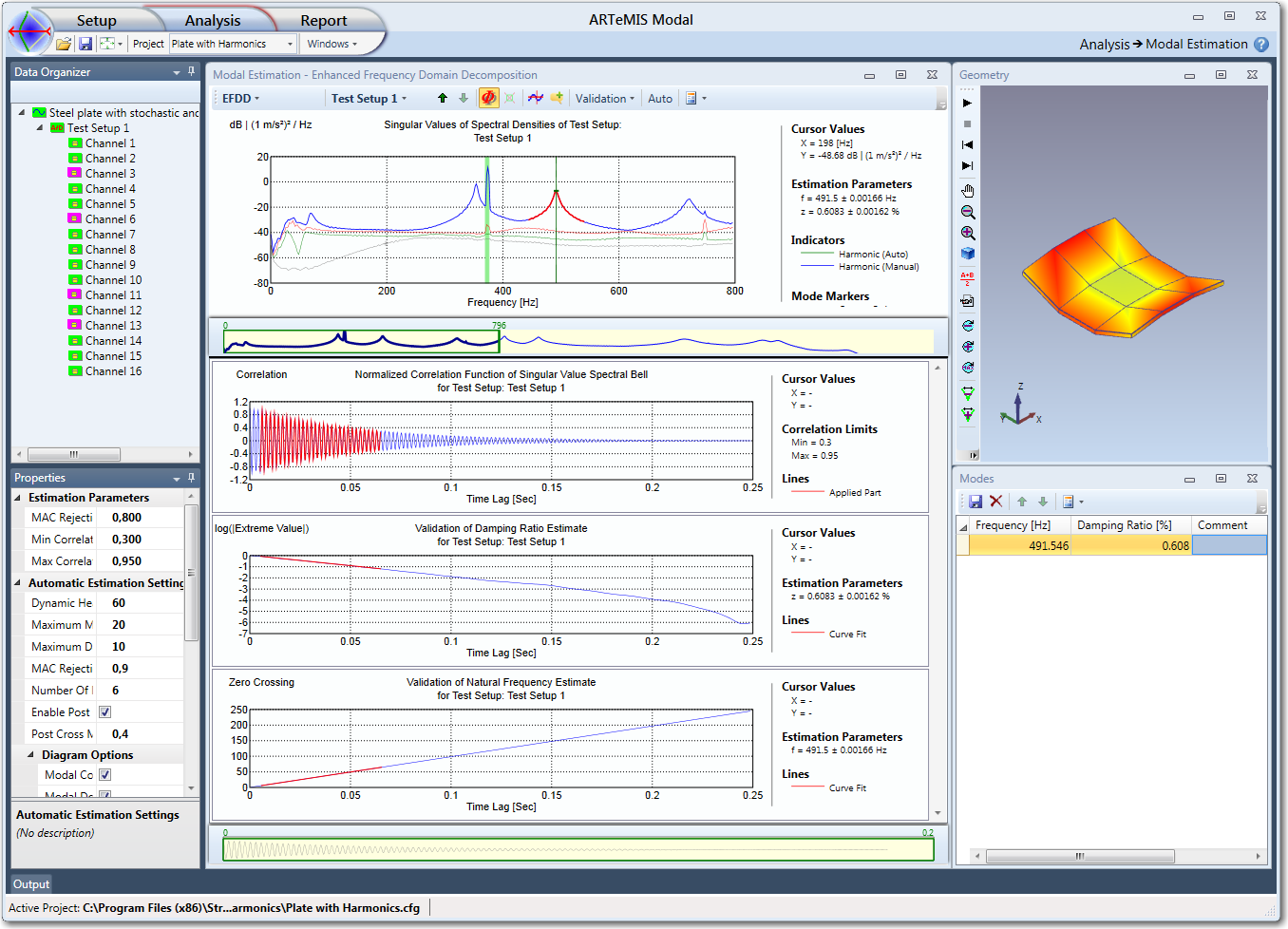
Here three windows appear allowing you to edit and validate the damping ratio and natural frequency estimates.

 

Normalized Correlation Function of Singular Value Spectral Bell Window

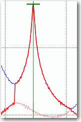
This window is located at the top of the three validation windows. The SDOF Spectral Bell is transformed using an algorithm based on the Fast Fourier Transform to obtain the SDOF Correlation Function that is normalized so it always start with the correlation 1. This function is what is presented in the this window.

The red region indicates the part of the correlation function that by default is used by the estimation algorithm. The choice of the maximum and minimum correlation limits to include is performed in the Properties window in the Estimation Parameters section. As default, it uses a maximum equal to 0.95. Now since the maximum correlation is 1 this means that the first values of the correlation function by default are excluded. This is because this part of the correlation function sometimes is polluted by a broad-banded noise. At the same time the minimum correlation limit is by default set at 0.3 because large time lags typically are estimated with increasing uncertainty.

Note: The correlation function here must look like in the above picture in order to be accurate. It is vital that it only consist of a single mode and not a mix of several (beating). If it is mixed try increase the MAC Rejection Level to filter out other modes.

 

Validation of Damping Ratio Estimate Window

This window is located as the mid window in the Validation window and its content is based on the SDOF Correlation function presented in the Normalized Correlation Function of Singular Value Spectral Bell Window as well as the maximum and minimum correlation limits selected in the Properties window under the Estimation Parameters section. This windows present the result of the regression leading to the damping ratio estimate.

The green curve presents the logarithm of the absolute value of all the positive and negative extremes. The red straight line is the result of the linear regression problem. The damping ratio can be found directly from the slope of this straight line. The standard deviation of the damping ratio is estimated by a linear transformation of the estimation error of the estimated slope.

 

Validation of Natural Frequency Estimate Window

This window is located in the bottom of the Validation window and its content is based on the SDOF Correlation function presented in the Normalized Correlation Function of Singular Value Spectral Bell Window as well as the maximum and minimum correlation limits selected in the Properties window under the Estimation Parameters section. This window presents the result of the regression leading to the natural frequency estimate.

This window is typically not important to check. The reason is that the zero-crossing times can be determined extremely accurately from the correlation function. In the above window they are presented as the green line. The result of the regression problem is presented as the red straight line. This regression result is based on the part of the correlation function that is inside the correlation limits. The natural frequency estimate is obtained from the slope of this estimated straight line as well as the estimated damping ratio.

Note: Because of the coupling of the regression problems the estimated standard deviation of the natural frequency depends on the estimation error of the slope of both regression
problems.